May 05, 2015

Bay Area Housing Price Heat Map

This is part of my research effort to find a home during this Apr/May period. Before that I never know there are 101 cities around San Francisco Bay Area …

The Result: Median Sale Price Heat Map

I think this median sale price is the most important affordability factor to consider of an area. And here is the median sale price by city - data at subdistrict level may represent a community more precisely than at city level…

Median Sale Price Heat Map

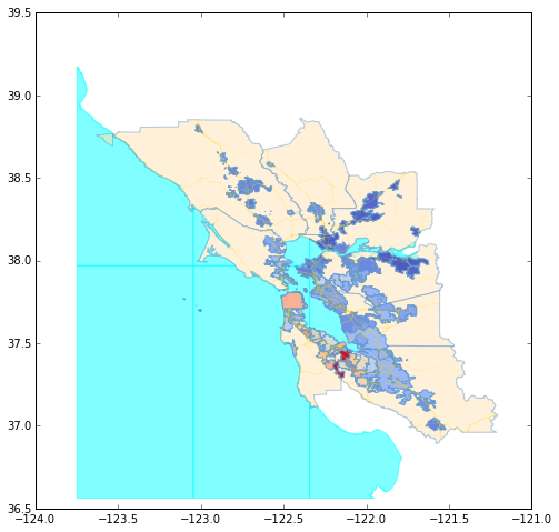
Pretty obviously, there are 2 centers in this “universe”, San Francisco and Palo Alto ;)

If you are more interested about exploring the data, you can stop here and there are quite a few websites that have pretty UI. and here are a few of them:

http://censusreporter.org
http://www.city-data.com
http://www.socialexplorer.com
http://factfinder.census.gov/

Following is my experience to craft the heat map…

Data Source

From the map we can see, we need the geography data and the housing price data. Thanks for the free and openness of America society, all these data can be obtained online without cost.

The city boundary data is from census.gov TIGER, there you can find geo map data at all administrative levels, County Subdivision, Elementary School District, …
For census data on top of these map, American Community Survey (ACS) has many interesting facts. I think this is the destination when the survey you filled when applying a Driver License or enrolling your child for the elementary school.
Bay Area is not a administrative area, I find some area map from SF OpenData
OpenStreetMap data can be extracted to work offline with metro extracts
There are housing price data from the government such as fhfa.org But I find zillow data is much more easier to work with - arguably, it is not that accurate.

Map Manipulation

Libaries I’ve used and recommended,

https://pypi.python.org/pypi/Fiona

Fiona reads and writes spatial data files

https://pypi.python.org/pypi/pyproj

Performs cartographic transformations and geodetic computations.

https://pypi.python.org/pypi/Shapely

Geometric objects, predicates, and operations

https://pypi.python.org/pypi/descartes

Use geometric objects as matplotlib paths and patches

Most of the geo data set either is in shapefile format or can be easily transform to the format. So if you model this process with Input/Process/Output, then you use Fiona to load the shapefile Input into memory; transform the coordination if multiple data source use different ones; process it with Shapely; then present the Output by transforming the geo objects to patches on matplotlib Axis with descartes.

If you don’t need to project the data on a earth globe, you don’t really need Basemap, Although you will find a lot hits with Google search. QGIS is the way to go if you need a full featured GIS system.

Code Example

When you got a shp file and you want to have a quick view what it looks like, you can load it to QGIS, or use tool like geovis.

But you can also write some code in ipython notebook and here it is.

import fiona
from shapely import geometry
from descartes.patch import PolygonPatch#, PathPatch
from matplotlib import cm
import matplotlib.colors as colors
import matplotlib.pyplot as plt

def plot_map(ax, source):
    norm = colors.Normalize(vmin=1, vmax=2*len(source))
    sm = cm.ScalarMappable(norm, cmap=cm.Paired)
    alpha, cnt = .8, 1
    for r in source:
        edge_color, color = sm.to_rgba(cnt), sm.to_rgba(cnt+1)
        cnt += 2
        shape = geometry.shape(r["geometry"])
        if isinstance(shape, geometry.Polygon):
            poly = shape
            ax.add_patch(PolygonPatch(poly, fc=color, ec=edge_color, alpha=alpha, zorder=1))
        elif isinstance(shape, geometry.MultiPolygon):
            for poly in shape:
                ax.add_patch(PolygonPatch(poly, fc=color, ec=edge_color, alpha=alpha, zorder=1))
        elif isinstance(shape, geometry.LineString):
            ax.plot(*shape.xy, color='gray', linewidth=3, solid_capstyle='round', zorder=1)
        elif isinstance(shape, geometry.MultiLineString):
            for line in shape:
                ax.plot(*line.xy, color='gray', linewidth=3, solid_capstyle='round', zorder=1)
        else:
            print r["geometry"]["type"]
            raise Exception("?")

## main ##
plt.rcParams['figure.figsize'] = (9, 16)
fig = plt.figure()
ax = fig.gca()

source_shapefile = "bayarea.map/city_land.shp"
with fiona.open(source_shapefile) as source:
    plot_map(ax, source)

ax.axis('scaled')
plt.show()

And github now rendering ipython notebook, you know? the above code rendering in github

Extended Reading

https://gis.stackexchange.com/questions/61862/simple-thematic-mapping-of-shapefile-using-python
http://www.geophysique.be/tutorials/
http://sensitivecities.com/so-youd-like-to-make-a-map-using-python-EN.html#.VRodn5NEW0c
http://nbviewer.ipython.org/github/mqlaql/geospatial-data/blob/master/Geospatial-Data-with-Python.ipynb
http://nbviewer.ipython.org/github/rjtavares/numbers_arent_people/blob/master/experiments/Plotting%20with%20Basemap%20and%20Shapefiles.ipynb
http://stackoverflow.com/questions/9128320/algorithm-buffer-effect-on-lines-other-geometric-shapes